Asymptotic Notations Pt 2

Big O Notation
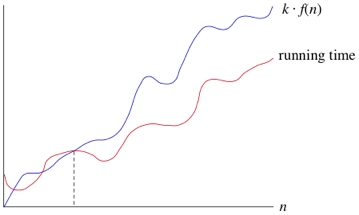
With the Big Theta notation we bound the growth of a runtime within a constant upper and lower factor. However, there are some times where we want to bound that growth to the upper factor. This is where the Big O notation comes in to play.

With binary search the worst case scenario is 𝛉(log2(n)), however, this is not the case 100% of the time as it is possible to find the target value on the first try which would make the runtime 𝛉(1). Therefore you can say that the runtime of binary search is never worse than 𝛉(log2(n)) but can be better. How would we write this using asymptotic notations, well we would write O(log2(n)).

Like with the big theta notation once n becomes large enough it is less than or equal to k * f(n), the big O notation can be used. Of course the Big O notation can also be used on any function and not just a logarithmic function.

Big Omega Notation

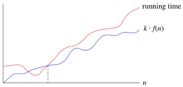
Sometimes we instead want to say that a runtime will take at least a certain amount of time, but without providing an upper bound. This is where the big omega notation comes into play. This means any function where n becomes large enough and is greater than or equal to k * f(n).

The Big Theta notation implies both Big O and Big Omega notations, but both Big O and Big Omega notations are imprecies due to not using both bounds. With this imprecision it is best to use Big Theta when describing a runtime of an algorithm.

Asymptotic Notations Pt 1

The runtime of any algorithm is decided by various factors such as the speed of the computer, the programming languages used, how long it takes for a compiler to translate the programming code into machine code and more.

We can think of the runtime of an algorithm as a function of the size of it's input. The makes sense when you look at linear or binary search algorithms because they take longer as you increase the size of the array that you are searching through.

We also need to think about the growth of the function as the size of the input increases, which is often referred to as the rate of growth. To make things more managable we simplify the function. This means removing the less important parts from the function. For example; we have the function 6n^2 + 100n + 300, where n is the size of the input. At some point the 6n^2 part of the function is going to become greater than 100n + 300 part, this actually happens when n = 20. Therefore we can get rid of the 100n + 300 part. We can also remove the 6 coefficient part of the 6n^2. This is because as long as the coefficient is > 0 then the difference will increase as does n. So we can say that the function grows as n^2.

By dropping the less important parts we can completely focus on the rate of growth of an algorithms runtime. When we do this we use asymptotic notations. Three examples of these types of notations are the big theta (𝛉), big O and big omega (𝛀).

Big Theta
As mentioned before the runtime of an algorithm is made up of various factors (some listed above) this will be denoted as c1. Then we have the input size or number of loop iterations, which is denoted as n. Finally we have the overhead of a function such as initialising the index to 0, this is denoted as c2. Using these values we can calculate the total time for the worst case scenario (which in a linear search is not finding a value). The formula is c1 * n + c2.

Both c1 and c2 don't tell us anything about the rate of growth of the runtime. The important part is n and so because both c1 and c2 are also constants we can drop both of them. Therefore the notation we use for the worst case scenario of a linear search is 𝛉(n).
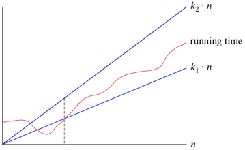
What this means is when n is large enough, the runtime is greater than k1 * n and less than k2 * n, where k1 and k2 are some constants. This can be seen in the graph below.

We can also use other functions of n, such as n^2 or nlog2. Therefore as long as any runtime that uses some function of n, f(n), is greater than k1 * f(n) and is less than k2 * f(n), it is a big theta notation or in other words 𝛉(f(n)).

Another advantage of using these notations means that we don't have to note the time units being used. So the previous example of 6n^2 + 100n + 300, becomes 𝛉(n^2). When we use this notation we are saying we have a asymptotically tight bound on the runtime. This is because it only matters when n is large enough (this gives us the asymptotically part) but also because the runtime is between the two k constants * f(n) (this gives us the tight bound part).

Growth Characteristics
There are 6 typical types of growth; constant, logarithmic, linear, linearithmic, polynomial and exponential, however, there are other types of growth that might not be covered.

An example of a constant growth is finding the first element within an array. The function would be 1 as element 0 is always the first element. An example of an logarithmic function is Log2(n). This means how many 2 we need to multiply to get n. Linear is where n (the size of the input) is multiplied by some sort of coefficient, for example 3n would have a linear growth. Linearithmic is a combination of logarithmic and linear functions. An example of this is nLog2(n). Polynomial is similar to linear but this time n has a power/indice that follows after it. For example 3n^2 or n^6. Finally there is exponential and this is where some number has an indice of n, for example (3/2)^n or 6^n.

The order of growth is:

1. Constant
2. Logarithmic
3. Linear
4. Linearithmic
5. Polynomial
6. Exponential

Its worth noting that with logarithmic and linearithmic functions the growth speed is dependant on the base, the lower the base value the quicker the growth. For example log2(n) is faster than log8(n). With polynomial and exponential functions, the higher value the power/indice is the quicker the growth. So n^2 is slower than n^4.

Precompiled Headers In C++

Usually when you include a header file in any C++ file, all of the contents of the header file is copied and compiled into the C++ file. This isn't so bad for a single header file, but if the header file also included several other header files, they also have to be compiled. So if you have a large project, you can expect the compile times to be very long without using precompiled headers. By precompiling headers, it converts a set of headers into a single file that uses the binary format in which the compiler can read and this is only done once. This however doesn't work if you add header files that you will be constantly or even occasionally changing as it means that the precompiled header now has to be recompiled every time a change is made.

Precompiled headers are usually used for headers that are going to be used often throughout the project such as the standard libary or any external libraries that you might be using. This is because they aren't going to change (unless there is a major issue with a version of an external library, which causes you to update that library). You can also use it for your own libraries but as mentioned above it is only worth doing if that library you have created is complete and isn't going to change or isn't likely to change.

There is a disadvantage to using precompiled headers and that is that it can hide the dependancies of a C++ file. Normally by just including whatever header files in a C++ file, you can easily tell what it requires. This means that if you were to reuse that C++ file within another project, you already know what else you will need if you don't already have it within that project. However, this is not the case with precompiled headers as it most likely has a ton of header files that are being used throughout the project but not specifically for the C++ file that you want to reuse. Therefore, if you did reuse that file you would have to figure out the header files that the file depends on.

Also if you are only going to use a header file in a single C++ file then it is not worth adding to the precompiled headers file. This is because that header file is more than likely going to be abstracted into your own api for you to use. An example of this would be the GLFW header file.

Below is a useful video on the subject, in which these notes are based on, but also the set up needed to use precompiled headers within a C++ project.

Enums Vs Enum Classes Pt 1

Enums and enum classes are essentially the same thing, however, using enum classes can avoid a compiler error as well as some other issues that maybe discussed in later posts.

enum AEnum
{
    OK,
    FAILED,
}

enum BEnum
{
    READY,
    FAILED,
}

The above enums will cause a compiler error and this is because within both enums the value FAILED has been declared twice as both values are within a global scope. By using enum classes instead avoids this problem as each value declared is now within its own enum class scope. A enum class is also known as a strongly typed enum. The below code shows the correct usage of enum classes. NB: Enum Classes are available in C++ 11+.

enum class AEnum
{
    OK,
    FAILED,
}

enum class BEnum
{
    READY,
    FAILED,
}

The Const Keyword: Const Functions

Const is generally used to state that something will not be changed or modified. However, this is dependant on where const is placed. For example if you place the const keyword after a member/class function declaration, you will not be allowed to modify any member variables within that function.

int GetMaxTries() const;

int GetMaxTries() const 
{
    return maxTries; 
}

The above function and function declaration will not produce any compiler errors as it doesn't modify any of the class's member variables. However, the below example would, because even with the const someone has tried to modify the maxTries variable. The const keyword in this situation acts as a guard so that you or anyone else working on the codebase doesn't accidentally modify any member variables within a specific function.

int GetMaxTries() const;

int GetMaxTries() const 
{
    maxTries += 12;
    return maxTries; 
}

Structs Vs Classes

Simply put structs and classes are the same except for one factor, which is, that all member variables and functions are public by default. This can be extremely useful. Below is an example of what a struct might look like and what a class might look like.

Struct Example

struct SomeStruct
{
    int someIntVariable;
    std::string someStringVariable;

    void SomeFunction();
}

Class Example

class SomeClass
{
public:
    SomeClass();
    ~SomeClass();

    void SomeFunction();
    int GetSomeIntVariable() { return someIntVariable; };

private:
    int someIntVariable;
}

Matrices Pt 3

Augmented Matrices
An augmented matrix is a matrix made of several linear equations that make up a system of equations. Each row of the matrix represents a equations within the system, whereas each column of the matrix represents a variable wtihin that equation.

We can see this with the above example, where we have two equations within a system and a matrix representation of that system. It also shows how the columns represents each variable or constant within the equation. For the x variables we have both 2 & 3, for y variables we have 5 & 4 and for the constant we have 10 & 24. This means we can write equations without having to write the x or y letters, or any other letters that might be used.

When converting a system of equations to a matrix, we need to make sure that each variable and constant is in line with each other but also if a variable or constant doesn't exist in one equation of the system then it defaults to 0 within the matrix at the location where the value would have gone.

Matrix Row Operators
There are three types of matrix row operators:

1. Switch any two rows
2. Multiply a row by a nonzero constant
3. Add one row to another

You will know to switch two rows of a matrix when given a question like R1 ↔ R2, which means swap row 1 with row 2. It is important to note that you can also subtract if needed.

You will know to multiply a row of a matrix by a nonzero constant when given a question like 3R1 → R1, which means multiply row 1 by 3. It is also important to note that you can essentially divide by a nonzero constant as well by using fractions like 1/2.

You will know to multiply a row of a matrix by a nonzero constant when given a question like R2 + R3 → R2, which means add row 2 to row 3 and enter the answer in row 2.

Each row operator could also be represented in this format:

On the left side we have the original matrix, in the center is the row operator and the direction being to the final matrix, which we can see on the right side.

It's also worth noting that they can be combined.

Notice how the 2R3 part only applies to the addition in row 1 and is not used to modify row 3.

As mentioned before augmented matrices represent a system of equations. By using row operators we can get equivelent systems of equations. For example by using the mutliplaction by a nonzero constant we can eliminate a variable from an equation.

This is our original system of equations and the augmented matrix. If we carried out -2R1 → R1, we get:

This then allows us to use the row addition operator; R1 + R2 → R2, which gives us:

In other words, we get the final equation -1y = -4, which we can use to solve for y. So y = 4, which can then be subsituted in any of the equations to solve for x.

Reduced Row Echelon Form
You can solve a system of equations by converting the augmented matrix into the reduced row echelon form. This form is were the diagonal components of a matrix are valued at 1 and every other component is valued at 0, except for any constants. Think of it being a combination of the identity matrix and an augmented matrix. Below is an example, where a, b & c are the constants.

To get to the reduced row echelon form, can use the row operators from earlier.

Once a augmented matrix has been converted we can solve the system of equations. So using the above example we can see that x = 5, y = -1 & z = -1 and if we subsitute them back into the original equations we can see that everything is correct.

1x + 1y + 1z = 3

1(5) + 1(-1) + 1(-1) = 3

5 - 1 -1 = 3